
[image] # Caption (optional) caption = “Image credit: Unsplash”
# Focal point (optional) # Options: Smart, Center, TopLeft, Top, TopRight, Left, Right, BottomLeft, Bottom, BottomRight focal_point = “”
Dependency
This post demonstrate the following:
- Quantile Normalization implemented in R package
preprocessCore. - Inverse-Normal-Transform implemented in
RNOmni
source("http://www.bioconductor.org/biocLite.R")
biocLite("preprocessCore")
install.packages("RNOmni")
library(preprocessCore)
library(RNOmni)General Princinples
Quantile Normalization
Simplest way to put it: Quantile normalization is a technique for making different distributions have the same statistical property by “aligning”" their quantiles. Statquest has a good video explaining this technique. Here is the video:
Inverse-Normal-Transform
Inverse normal transformation, a.k.a ranked based Inverse-Normal-Transformation(INT), is a theoretically complicated method. But again, the simplest way to put it: INT increase the “normality” of the distribution, by aligning the quantiles to the standard normal quantiles. As a result we can now apply statistal models that have a normality assumption.
Be Cautious!
Normalization techeniques are highly application specific. Blindly appling them may create as many problems as they solve. If you don’t know the “right”" one to use, you’d better do some test-ride and select the one that is statistically better(e.g. Cross-Validation, etc.).
Set plot parameters
library(RColorBrewer)
qual_col_pals = brewer.pal.info[brewer.pal.info$category == 'qual',]
col_vec = unlist(mapply(brewer.pal, qual_col_pals$maxcolors, rownames(qual_col_pals))) # 74 colors in RcolorBrewer
Load Data
The data in this post is a data.frame where rows are genes and columns are patients, the measurement is \(log_2(rpkm + 1)\). It’s straghtforward to understand so I’d rather not to bother to provide a link for it.
data = read.csv("/Users/bos/R-workspace/2.eQTL/large500_expr")
expr = as.matrix(data[,-1])  # 1st column is gene id
Quantile Transformation
before quantile transformation
plot(density(unlist(expr[, 1])), col=col_vec[1])
for(i in 2:40) lines(density(expr[,i]), col=col_vec[i])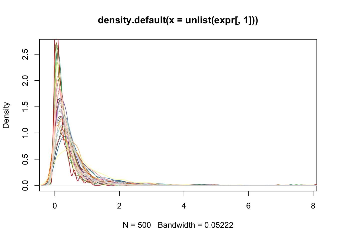
after quantile transformation
expr.qt <- preprocessCore::normalize.quantiles(as.matrix(expr))
plot(density(expr.qt[,1]), col = col_vec[1])
for(i in 2:40) lines(density(expr.qt[,i]), col=col_vec[i])
Note here most part of those transformed distributions land on top of each other, but if the variability is larger in your data, then near the tail the distributions will not be perfectly same which is good because it keeps the variability.
However, Quantile Normalization can not remove batch effect, see Jeff’s post
Inverse-Normal-Transformation
before
plot(density(expr[1,]), col = col_vec[1])
for(i in 2:40) lines(density(expr[i, ]), col = col_vec[i])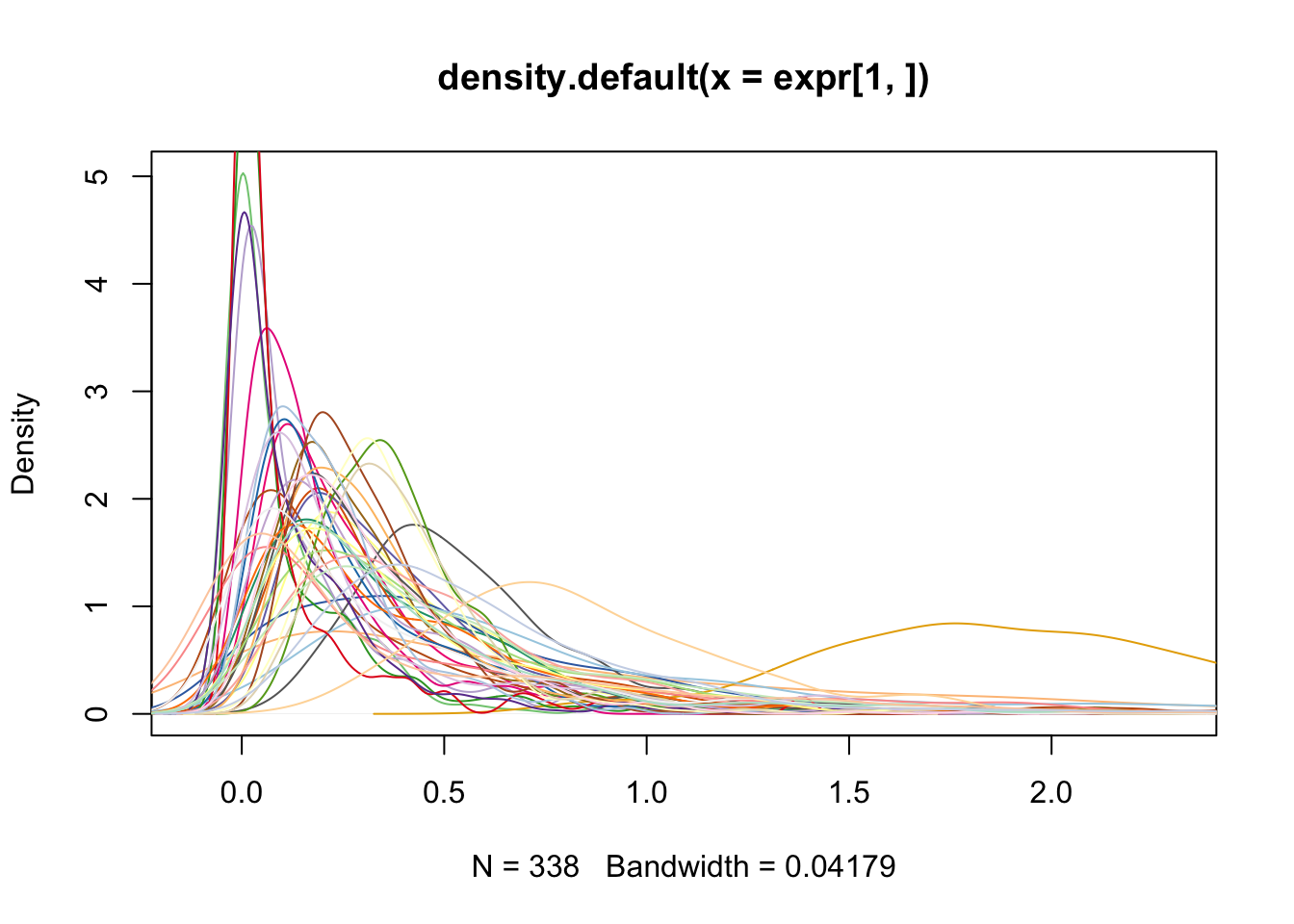
After
expr.int = t(apply(expr, 1, RNOmni::rankNormal))
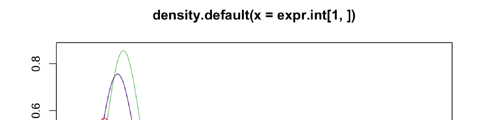
plot(density(expr.int[1,]), col = col_vec[1])
for(i in 2:40) lines(density(expr.int[i, ]), col = col_vec[i])
As you can see, the distribution are normalized toward std. normal, and variability of the tails are preserved.(You may expect a different result with this plot, because my data here is RNA-seq data with heavy-tails, for moderate-tailed data, it should become more similar to a std. normal. )
Session Information
if (!requireNamespace("devtools")) install.packages("devtools")## Loading required namespace: devtoolsdevtools::session_info()## Session info -------------------------------------------------------------## setting value
## version R version 3.5.0 (2018-04-23)
## system x86_64, darwin15.6.0
## ui X11
## language (EN)
## collate en_US.UTF-8
## tz America/Los_Angeles
## date 2018-10-20## Packages -----------------------------------------------------------------## package * version date source
## abind 1.4-5 2016-07-21 CRAN (R 3.5.0)
## backports 1.1.2 2017-12-13 CRAN (R 3.5.0)
## base * 3.5.0 2018-04-24 local
## blogdown 0.8 2018-07-15 CRAN (R 3.5.0)
## bookdown 0.7 2018-02-18 CRAN (R 3.5.0)
## codetools 0.2-15 2016-10-05 CRAN (R 3.5.0)
## compiler 3.5.0 2018-04-24 local
## datasets * 3.5.0 2018-04-24 local
## devtools 1.13.6 2018-06-27 CRAN (R 3.5.0)
## digest 0.6.15 2018-01-28 CRAN (R 3.5.0)
## evaluate 0.11 2018-07-17 CRAN (R 3.5.0)
## foreach 1.4.4 2017-12-12 CRAN (R 3.5.0)
## graphics * 3.5.0 2018-04-24 local
## grDevices * 3.5.0 2018-04-24 local
## htmltools 0.3.6 2017-04-28 CRAN (R 3.5.0)
## iterators 1.0.10 2018-07-13 CRAN (R 3.5.0)
## knitr 1.20 2018-02-20 CRAN (R 3.5.0)
## magrittr 1.5 2014-11-22 CRAN (R 3.5.0)
## memoise 1.1.0 2017-04-21 CRAN (R 3.5.0)
## methods * 3.5.0 2018-04-24 local
## plyr 1.8.4 2016-06-08 CRAN (R 3.5.0)
## preprocessCore * 1.42.0 2018-05-01 Bioconductor
## RColorBrewer * 1.1-2 2014-12-07 CRAN (R 3.5.0)
## Rcpp 0.12.18 2018-07-23 cran (@0.12.18)
## rmarkdown 1.10 2018-06-11 CRAN (R 3.5.0)
## RNOmni * 0.4.0 2018-05-16 CRAN (R 3.5.0)
## rprojroot 1.3-2 2018-01-03 CRAN (R 3.5.0)
## stats * 3.5.0 2018-04-24 local
## stringi 1.2.4 2018-07-20 CRAN (R 3.5.0)
## stringr 1.3.1 2018-05-10 CRAN (R 3.5.0)
## tools 3.5.0 2018-04-24 local
## utils * 3.5.0 2018-04-24 local
## withr 2.1.2 2018-03-15 CRAN (R 3.5.0)
## xfun 0.3 2018-07-06 CRAN (R 3.5.0)
## yaml 2.2.0 2018-07-25 CRAN (R 3.5.0)